HDA Flowsheet Simulation and Optimization

HDA Flowsheet Simulation and Optimization#

Author: Jaffer Ghouse
Maintainer: Tanner Polley
Updated: 2025-06-03

Learning outcomes#

Construct a steady-state flowsheet using the IDAES unit model library
Connecting unit models in a flowsheet using Arcs
Using the SequentialDecomposition tool to initialize a flowsheet with recycle
Formulate and solve an optimization problem
- Defining an objective function
- Setting variable bounds
- Adding additional constraints

The general workflow of setting up an IDAES flowsheet is the following:

     1 Importing Modules
     2 Building a Model
     3 Scaling the Model
     4 Specifying the Model
     5 Initializing the Model
     6 Solving the Model
     7 Analyzing and Visualizing the Results
     8 Optimizing the Model

We will complete each of these steps as well as demonstrate analyses on this model through some examples and exercises.

Problem Statement#

Hydrodealkylation is a chemical reaction that often involves reacting an aromatic hydrocarbon in the presence of hydrogen gas to form a simpler aromatic hydrocarbon devoid of functional groups. In this example, toluene will be reacted with hydrogen gas at high temperatures to form benzene via the following reaction:

C₆H₅CH₃ + H₂ → C₆H₆ + CH₄

This reaction is often accompanied by an equilibrium side reaction which forms diphenyl, which we will neglect for this example.

This example is based on the 1967 AIChE Student Contest problem as present by Douglas, J.M., Chemical Design of Chemical Processes, 1988, McGraw-Hill.

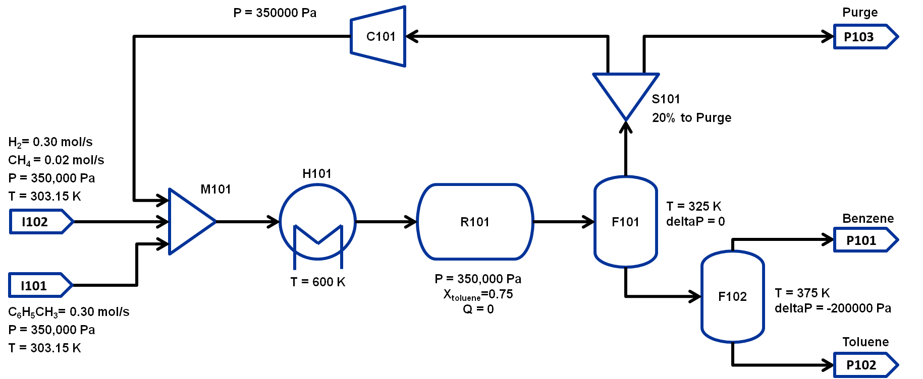
The flowsheet that we will be using for this module is shown below with the stream conditions. We will be processing toluene and hydrogen to produce at least 370 TPY of benzene. As shown in the flowsheet, there are two flash tanks, F101 to separate out the non-condensibles and F102 to further separate the benzene-toluene mixture to improve the benzene purity. Note that typically a distillation column is required to obtain high purity benzene but that is beyond the scope of this workshop. The non-condensibles separated out in F101 will be partially recycled back to M101 and the rest will be either purged or combusted for power generation.We will assume ideal gas for this flowsheet. The properties required for this module are available in the same directory:

hda_ideal_VLE.py
hda_reaction.py

The state variables chosen for the property package are flows of component by phase, temperature and pressure. The components considered are: toluene, hydrogen, benzene and methane. Therefore, every stream has 8 flow variables, 1 temperature and 1 pressure variable.

1 Importing Modules#

1.1 Importing required Pyomo and IDAES components#

To construct a flowsheet, we will need several components from the Pyomo and IDAES package. Let us first import the following components from Pyomo:

Constraint (to write constraints)
Var (to declare variables)
ConcreteModel (to create the concrete model object)
Expression (to evaluate values as a function of variables defined in the model)
Objective (to define an objective function for optimization)
SolverFactory (to solve the problem)
TransformationFactory (to apply certain transformations)
Arc (to connect two unit models)
SequentialDecomposition (to initialize the flowsheet in a sequential mode)

For further details on these components, please refer to the Pyomo documentation: https://Pyomo.readthedocs.io/en/stable/

from pyomo.environ import (
    Constraint,
    Var,
    ConcreteModel,
    Expression,
    Objective,
    SolverFactory,
    TransformationFactory,
    value,
)
from pyomo.network import Arc, SequentialDecomposition

From IDAES, we will be needing the FlowsheetBlock and the following unit models:

Feed
Mixer
Heater
StoichiometricReactor
Flash
Separator (splitter)
PressureChanger
Product

from idaes.core import FlowsheetBlock

from idaes.models.unit_models import (
    PressureChanger,
    IsentropicPressureChangerInitializer,
    Mixer,
    MixerInitializer,
    Separator as Splitter,
    SeparatorInitializer,
    Heater,
    StoichiometricReactor,
    Feed,
    Product,
)

Inline Exercise: Now, import the remaining unit models highlighted in blue above and run the cell using `Shift+Enter` after typing in the code.

# Todo: import flash model from idaes.models.unit_models
from idaes.models.unit_models import Flash

We will also be needing some utility tools to put together the flowsheet and calculate the degrees of freedom.

from idaes.models.unit_models.pressure_changer import ThermodynamicAssumption
from idaes.core.util.model_statistics import degrees_of_freedom
from idaes.core.scaling.util import set_scaling_factor
from idaes.core.scaling.autoscaling import AutoScaler

# Import idaes logger to set output levels
import idaes.logger as idaeslog
from idaes.core.solvers import get_solver
from idaes.core.util.exceptions import InitializationError

1.2 Importing required thermo and reaction package#

The final set of imports are to import the thermo and reaction package for the HDA process. We have created a custom thermo package that assumes Ideal Gas with support for VLE.

The reaction package here is very simple as we will be using only a StochiometricReactor and the reaction package consists of the stochiometric coefficients for the reaction and the parameter for the heat of reaction.

Let us import the following modules and they are in the same directory as this jupyter notebook:

hda_ideal_VLE as thermo_props
hda_reaction as reaction_props

from idaes_examples.mod.hda import hda_ideal_VLE as thermo_props
from idaes_examples.mod.hda import hda_reaction as reaction_props

2 Constructing the Flowsheet#

We have now imported all the components, unit models, and property modules we need to construct a flowsheet. Let us create a ConcreteModel and add the flowsheet block.

m = ConcreteModel()
m.fs = FlowsheetBlock(dynamic=False)

We now need to add the property packages to the flowsheet. Unlike Module 1, where we only had a thermo property package, for this flowsheet we will also need to add a reaction property package.

m.fs.thermo_params = thermo_props.HDAParameterBlock()
m.fs.reaction_params = reaction_props.HDAReactionParameterBlock(
    property_package=m.fs.thermo_params
)

2.1 Adding Unit Models#

Let us start adding the unit models we have imported to the flowsheet. Here, we are adding the Feed (assigned a name I101 for Inlet), Mixer (assigned a name M101) and a Heater (assigned a name H101). Note that, all unit models need to be given a property package argument. In addition to that, there are several arguments depending on the unit model, please refer to the documentation for more details (https://idaes-pse.readthedocs.io/en/stable/reference_guides/model_libraries/generic/unit_models/index.html). For example, the Mixer unit model here must be specified the number of inlets that it will take in and the Heater can have specific settings enabled such as has_pressure_change or has_phase_equilibrium.

m.fs.I101 = Feed(property_package=m.fs.thermo_params)

m.fs.I102 = Feed(property_package=m.fs.thermo_params)

m.fs.M101 = Mixer(
    property_package=m.fs.thermo_params,
    num_inlets=3,
)

m.fs.H101 = Heater(
    property_package=m.fs.thermo_params,
    has_pressure_change=False,
    has_phase_equilibrium=True,
)

# Todo: Add reactor with the specifications above
m.fs.R101 = StoichiometricReactor(
    property_package=m.fs.thermo_params,
    reaction_package=m.fs.reaction_params,
    has_heat_of_reaction=True,
    has_heat_transfer=True,
    has_pressure_change=False,
)

Let us now add the Flash(assign the name F101) and pass the following arguments:

”property_package”: m.fs.thermo_params
”has_heat_transfer”: True
”has_pressure_change”: False

m.fs.F101 = Flash(
    property_package=m.fs.thermo_params,
    has_heat_transfer=True,
    has_pressure_change=True,
)

Let us now add the Splitter(S101) with specific names for its output (purge and recycle), PressureChanger(C101) and the second Flash(F102).

m.fs.S101 = Splitter(
    property_package=m.fs.thermo_params,
    ideal_separation=False,
    outlet_list=["purge", "recycle"],
)


m.fs.C101 = PressureChanger(
    property_package=m.fs.thermo_params,
    compressor=True,
    thermodynamic_assumption=ThermodynamicAssumption.isothermal,
)

m.fs.F102 = Flash(
    property_package=m.fs.thermo_params,
    has_heat_transfer=True,
    has_pressure_change=True,
)

Last, we will add the three Product blocks (P101, P102, P103). We use Feed blocks and Product blocks for convenience with reporting stream summaries and consistency

m.fs.P101 = Product(property_package=m.fs.thermo_params)

m.fs.P102 = Product(property_package=m.fs.thermo_params)

m.fs.P103 = Product(property_package=m.fs.thermo_params)

2.2 Connecting Unit Models using Arcs#

We have now added all the unit models we need to the flowsheet. However, we have not yet specified how the units are to be connected. To do this, we will be using the Arc which is a Pyomo component that takes in two arguments: source and destination. Let us connect the outlet of the inlets (I101, I102) to the inlet of the mixer (M101) and outlet of the mixer to the inlet of the heater(H101).

m.fs.s01 = Arc(source=m.fs.I101.outlet, destination=m.fs.M101.inlet_1)
m.fs.s02 = Arc(source=m.fs.I102.outlet, destination=m.fs.M101.inlet_2)
m.fs.s03 = Arc(source=m.fs.M101.outlet, destination=m.fs.H101.inlet)

# Todo: Connect the H101 outlet to R101 inlet
m.fs.s04 = Arc(source=m.fs.H101.outlet, destination=m.fs.R101.inlet)

We will now be connecting the rest of the flowsheet as shown below. Notice how the outlet names are different for the flash tanks F101 and F102 as they have a vapor and a liquid outlet.

m.fs.s05 = Arc(source=m.fs.R101.outlet, destination=m.fs.F101.inlet)
m.fs.s06 = Arc(source=m.fs.F101.vap_outlet, destination=m.fs.S101.inlet)
m.fs.s07 = Arc(source=m.fs.F101.liq_outlet, destination=m.fs.F102.inlet)
m.fs.s08 = Arc(source=m.fs.S101.recycle, destination=m.fs.C101.inlet)
m.fs.s09 = Arc(source=m.fs.C101.outlet, destination=m.fs.M101.inlet_3)

Last we will connect the outlet streams to the inlets of the Product blocks (P101, P102, P103)

m.fs.s10 = Arc(source=m.fs.F102.vap_outlet, destination=m.fs.P101.inlet)
m.fs.s11 = Arc(source=m.fs.F102.liq_outlet, destination=m.fs.P102.inlet)
m.fs.s12 = Arc(source=m.fs.S101.purge, destination=m.fs.P103.inlet)

We have now connected the unit model block using the arcs. However, each of these arcs link to ports on the two unit models that are connected. In this case, the ports consist of the state variables that need to be linked between the unit models. Pyomo provides a convenient method to write these equality constraints for us between two ports and this is done as follows:

TransformationFactory("network.expand_arcs").apply_to(m)

2.3 Adding expressions to compute purity and operating costs#

In this section, we will add a few Expressions that allows us to evaluate the performance. Expressions provide a convenient way of calculating certain values that are a function of the variables defined in the model. For more details on Expressions, please refer to: https://pyomo.readthedocs.io/en/stable/explanation/modeling/network.html.

For this flowsheet, we are interested in computing the purity of the product Benzene stream (i.e. the mole fraction) and the operating cost which is a sum of the cooling and heating cost.

Let us first add an Expression to compute the mole fraction of benzene in the vap_outlet of F102 which is our product stream. Please note that the var flow_mol_phase_comp has the index - [time, phase, component]. As this is a steady-state flowsheet, the time index by default is 0. The valid phases are [“Liq”, “Vap”]. Similarly the valid component list is [“benzene”, “toluene”, “hydrogen”, “methane”].

m.fs.purity = Expression(
    expr=m.fs.F102.vap_outlet.flow_mol_phase_comp[0, "Vap", "benzene"]
    / (
        m.fs.F102.vap_outlet.flow_mol_phase_comp[0, "Vap", "benzene"]
        + m.fs.F102.vap_outlet.flow_mol_phase_comp[0, "Vap", "toluene"]
    )
)

Now, let us add an expression to compute the cooling cost assuming a cost of 0.212E-4 $/kW. Note that cooling utility is required for the reactor (R101) and the first flash (F101).

m.fs.cooling_cost = Expression(
    expr=0.212e-7 * (-m.fs.F101.heat_duty[0]) + 0.212e-7 * (-m.fs.R101.heat_duty[0])
)

Now, let us add an expression to compute the heating cost assuming the utility cost as follows:

2.2E-4 dollars/kW for H101
1.9E-4 dollars/kW for F102

Note that the heat duty is in units of watt (J/s).

m.fs.heating_cost = Expression(
    expr=2.2e-7 * m.fs.H101.heat_duty[0] + 1.9e-7 * m.fs.F102.heat_duty[0]
)

Let us now add an expression to compute the total operating cost per year which is basically the sum of the cooling and heating cost we defined above.

m.fs.operating_cost = Expression(
    expr=(3600 * 24 * 365 * (m.fs.heating_cost + m.fs.cooling_cost))
)

3 Scaling the Model#

In this example, we will simply use the AutoScaler method to scale our model since this example is focused on introductory flowsheet building for a full process system.

For more direct control, a manual, magnitude based approach can be used. If this method is chosen or appropriate, it is highly recommended to look at these documentation:

Scaling Toolbox https://idaes-pse.readthedocs.io/en/stable/reference_guides/scaling/scaling.html
Scaling Workshop https://idaes-examples.readthedocs.io/en/latest/docs/scaling/scaler_workshop_doc.html.

In this example, we already imported the AutoScaler class in the beginning so we just create the autoscaler object and call the scale_model method on the model m.

autoscaler = AutoScaler()
autoscaler.scale_model(m)

WARNING: model contains export suffix 'scaling_factor' that contains 2
component keys that are not exported as part of the NL file.  Skipping.

4 Specifying the Model#

4.1 Fixing feed conditions#

Let us first check how many degrees of freedom exist for this flowsheet using the degrees_of_freedom tool we imported earlier.

print(degrees_of_freedom(m))

We will now be fixing the toluene feed (I101) stream to the conditions shown in the flowsheet above. Please note that though this is a pure toluene feed, the remaining components are still assigned a very small non-zero value to help with convergence and initializing.

m.fs.I101.flow_mol_phase_comp[0, "Vap", "benzene"].fix(1e-5)
m.fs.I101.flow_mol_phase_comp[0, "Vap", "toluene"].fix(1e-5)
m.fs.I101.flow_mol_phase_comp[0, "Vap", "hydrogen"].fix(1e-5)
m.fs.I101.flow_mol_phase_comp[0, "Vap", "methane"].fix(1e-5)
m.fs.I101.flow_mol_phase_comp[0, "Liq", "benzene"].fix(1e-5)
m.fs.I101.flow_mol_phase_comp[0, "Liq", "toluene"].fix(0.30)
m.fs.I101.flow_mol_phase_comp[0, "Liq", "hydrogen"].fix(1e-5)
m.fs.I101.flow_mol_phase_comp[0, "Liq", "methane"].fix(1e-5)
m.fs.I101.temperature.fix(303.2)
m.fs.I101.pressure.fix(350000)

Similarly, let us fix the hydrogen feed (I102) to the following conditions in the next cell:

F_H2 = 0.30 mol/s
F_CH4 = 0.02 mol/s
Remaining components = 1e-5 mol/s
T = 303.2 K
P = 350000 Pa

m.fs.I102.flow_mol_phase_comp[0, "Vap", "benzene"].fix(1e-5)
m.fs.I102.flow_mol_phase_comp[0, "Vap", "toluene"].fix(1e-5)
m.fs.I102.flow_mol_phase_comp[0, "Vap", "hydrogen"].fix(0.30)
m.fs.I102.flow_mol_phase_comp[0, "Vap", "methane"].fix(0.02)
m.fs.I102.flow_mol_phase_comp[0, "Liq", "benzene"].fix(1e-5)
m.fs.I102.flow_mol_phase_comp[0, "Liq", "toluene"].fix(1e-5)
m.fs.I102.flow_mol_phase_comp[0, "Liq", "hydrogen"].fix(1e-5)
m.fs.I102.flow_mol_phase_comp[0, "Liq", "methane"].fix(1e-5)
m.fs.I102.temperature.fix(303.2)
m.fs.I102.pressure.fix(350000)

4.2 Fixing unit model specifications#

Now that we have fixed our inlet feed conditions, we will now be fixing the operating conditions for the unit models in the flowsheet. Let us set set the H101 outlet temperature to 600 K.

m.fs.H101.outlet.temperature.fix(600)

For the StoichiometricReactor, we have to define the conversion in terms of toluene. This requires us to create a new variable for specifying the conversion and adding a Constraint that defines the conversion with respect to toluene. The second degree of freedom for the reactor is to define the heat duty. In this case, let us assume the reactor to be adiabatic i.e. Q = 0.

m.fs.R101.conversion = Var(initialize=0.75, bounds=(0, 1))

m.fs.R101.conv_constraint = Constraint(
    expr=m.fs.R101.conversion * m.fs.R101.inlet.flow_mol_phase_comp[0, "Vap", "toluene"]
    == (
        m.fs.R101.inlet.flow_mol_phase_comp[0, "Vap", "toluene"]
        - m.fs.R101.outlet.flow_mol_phase_comp[0, "Vap", "toluene"]
    )
)

m.fs.R101.conversion.fix(0.75)
m.fs.R101.heat_duty.fix(0)

The Flash conditions for F101 can be set as follows.

m.fs.F101.vap_outlet.temperature.fix(325.0)
m.fs.F101.deltaP.fix(0)

m.fs.F102.vap_outlet.temperature.fix(375)
m.fs.F102.deltaP.fix(-200000)

Let us fix the purge split fraction to 20% and the outlet pressure of the compressor is set to 350000 Pa.

m.fs.S101.split_fraction[0, "purge"].fix(0.2)
m.fs.C101.outlet.pressure.fix(350000)

print(degrees_of_freedom(m))

5 Initializing the Model#

When a flowsheet contains a recycle loop, the outlet of a downstream unit becomes the inlet of an upstream unit, creating a cyclic dependency that prevents straightforward calculation of all stream conditions. The tear‐stream method is necessary because it “breaks” this loop: you select one recycle stream as the tear, assign it an initial guess, and then solve the rest of the flowsheet as if it were acyclic. Once the downstream units compute their outputs, you compare the calculated value of the torn stream to your initial guess and iteratively adjust until they coincide. Without tearing, the solver cannot establish a proper topological sequence or drive the recycle to convergence, making initialization—and ultimately steady‐state convergence—impossible.

It is important to determine the tear stream for a flowsheet which will be demonstrated below.

Currently, there are two methods of initializing a full flowsheet: using the sequential decomposition tool, or manually propagating through the flowsheet. Both methods will be shown.

5.1 Sequential Decomposition#

This section will demonstrate how to use the built-in sequential decomposition tool to initialize our flowsheet. Sequential Decomposition is a tool from Pyomo where the documentation can be found here https://Pyomo.readthedocs.io/en/stable/explanation/modeling/network.html#sequential-decomposition

Let us first create an object for the SequentialDecomposition and specify our options for this. We can also create a graph for our flowsheet to determine the tear set and order.

seq = SequentialDecomposition()
seq.options.select_tear_method = "heuristic"
seq.options.tear_method = "Wegstein"
seq.options.iterLim = 3

# Using the SD tool
G = seq.create_graph(m)
heuristic_tear_set = seq.tear_set_arcs(G, method="heuristic")
order = seq.calculation_order(G)

Which is the tear stream? Display tear set and order

for o in heuristic_tear_set:
    print(o.name)

fs.s03

What sequence did the SD tool determine to solve this flowsheet with the least number of tears?

for o in order:
    print(o[0].name)

fs.I101
fs.R101
fs.F101
fs.S101
fs.C101
fs.M101

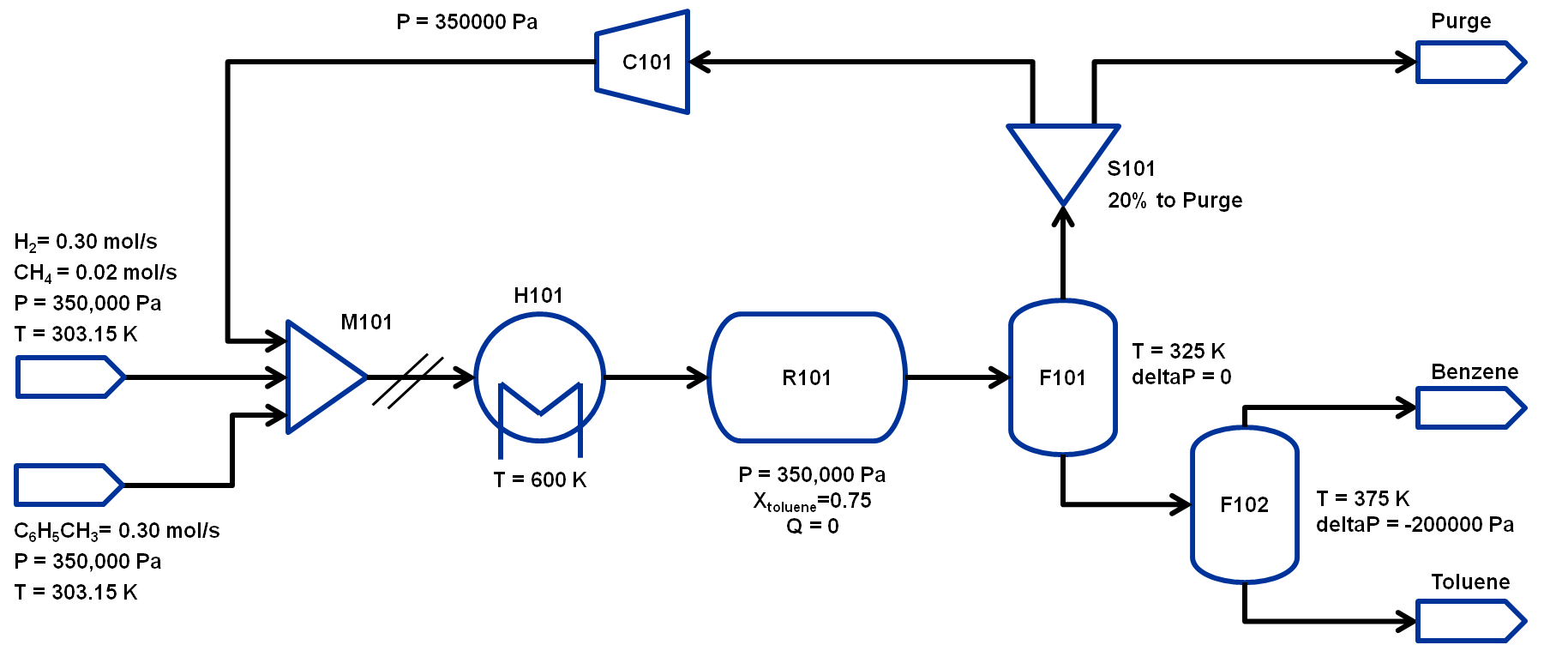
The SequentialDecomposition tool has determined that the tear stream is the mixer outlet. You can see this shown in the picture of the flowsheet above as the outlet of the mixer as the two lines crossing it identifying it as the tear stream. We will need to provide a reasonable guess for this.

tear_guesses = {
    "flow_mol_phase_comp": {
        (0, "Liq", "benzene"): 1e-5,
        (0, "Liq", "toluene"): 0.30,
        (0, "Liq", "methane"): 1e-5,
        (0, "Liq", "hydrogen"): 1e-5,
        (0, "Vap", "benzene"): 1e-5,
        (0, "Vap", "toluene"): 1e-5,
        (0, "Vap", "methane"): 0.02,
        (0, "Vap", "hydrogen"): 0.30,
    },
    "temperature": {0: 303},
    "pressure": {0: 350000},
}

# Pass the tear_guess to the SD tool
seq.set_guesses_for(m.fs.H101.inlet, tear_guesses)

Next, we need to tell the tool how to initialize a particular unit. We will be writing a python function which takes in a “unit” and calls the initialize method on that unit.

def function(unit):
    try:
        initializer = unit.default_initializer()
        initializer.initialize(unit, output_level=idaeslog.INFO)
    except InitializationError:
        solver = get_solver()
        solver.solve(unit)

We are now ready to initialize our flowsheet in a sequential mode. Note that we specifically set the iteration limit to be 5 as we are trying to use this tool only to get a good set of initial values such that IPOPT can then take over and solve this flowsheet for us.

# seq.run(m, function)

5.2 Manual Propagation Method#

This method uses a more direct approach to initialize the flowsheet, utilizing the updated initializer method and propagating manually through the flowsheet and solving for the tear stream directly. Lets first import a helper function that will help us manually propagate and step through the flowsheet

from idaes.core.util.initialization import propagate_state

Now we can setup our initial guesses for the tear stream which we know is the outlet of the Mixer or the inlet of the Heater. We can use the same initial guesses used in the first method. We also want to ensure that the degrees of freedom are consistent while we manually initialize the model.

We will first ensure that are current degrees of freedom is still zero

print(f"The DOF is {degrees_of_freedom(m)} initially")

The DOF is 0 initially

Now we can manually deactivate the tear stream, creating a separation between the Mixer and Heater. This should reduce the degrees of freedom by 10 since the inlet of the Heater now contains no values to solve the unit model. To deactivate a stream, simply use m.fs.s03_expanded.deactivate(). This expanded stream is just a different version of the Arc stream that is able to be deactivated.

m.fs.s03_expanded.deactivate()

print(f"The DOF is {degrees_of_freedom(m)} after deactivating the tear stream")

The DOF is 10 after deactivating the tear stream

Now we can provide the Heater inlet 10 guess values to bring the degrees of freedom back to 0 and start the manual initialization process. We can run this convenient loop to assign each of these guesses to the inlet of the heater.

tear_guesses = {
    "flow_mol_phase_comp": {
        (0, "Liq", "benzene"): 1e-5,
        (0, "Liq", "toluene"): 0.30,
        (0, "Liq", "methane"): 1e-5,
        (0, "Liq", "hydrogen"): 1e-5,
        (0, "Vap", "benzene"): 1e-5,
        (0, "Vap", "toluene"): 1e-5,
        (0, "Vap", "methane"): 0.5,
        (0, "Vap", "hydrogen"): 0.5,
    },
    "temperature": {0: 303},
    "pressure": {0: 350000},
}

for k, v in tear_guesses.items():
    for k1, v1 in v.items():
        getattr(m.fs.s03.destination, k)[k1].fix(v1)

DOF_initial = degrees_of_freedom(m)
print(f"The DOF is {degrees_of_freedom(m)} after providing the initial guesses")

The DOF is 0 after providing the initial guesses

The next step is to manually initialize each unit model starting from the Heater and then propagate the connection between it and the next unit model. This manual process ensures a strict order to the user’s specification if that is desired. The current standard for initializing a unit model is to use an initializer object most compatible for that unit model. This can most often be done by utilizing the default_initializer() method attached to the unit model and then to call the initialize() method with the unit model as the argument.

m.fs.H101.default_initializer().initialize(m.fs.H101)  # Initialize Heater
propagate_state(m.fs.s04)  # Establish connection between Heater and Reactor
m.fs.R101.default_initializer().initialize(m.fs.R101)  # Initialize Reactor
propagate_state(m.fs.s05)  # Establish connection between Reactor and First Flash Unit
m.fs.F101.default_initializer().initialize(m.fs.F101)  # Initialize First Flash Unit
propagate_state(m.fs.s06)  # Establish connection between First Flash Unit and Splitter
propagate_state(
    m.fs.s07
)  # Establish connection between First Flash Unit and Second Flash Unit
m.fs.S101.default_initializer().initialize(m.fs.S101)  # Initialize Splitter
propagate_state(m.fs.s08)  # Establish connection between Splitter and Compressor
m.fs.C101.default_initializer().initialize(m.fs.C101)  # Initialize Compressor
propagate_state(m.fs.s09)  # Establish connection between Compressor and Mixer
m.fs.I101.default_initializer().initialize(m.fs.I101)  # Initialize Toluene Inlet
propagate_state(m.fs.s01)  # Establish connection between Toluene Inlet and Mixer
m.fs.I102.default_initializer().initialize(m.fs.I102)  # Initialize Hydrogen Inlet
propagate_state(m.fs.s02)  # Establish connection between Hydrogen Inlet and Mixer
m.fs.M101.default_initializer().initialize(m.fs.M101)  # Initialize Mixer
propagate_state(m.fs.s03)  # Establish connection between Mixer and Heater
m.fs.F102.default_initializer().initialize(m.fs.F102)  # Initialize Second Flash Unit
propagate_state(
    m.fs.s10
)  # Establish connection between Second Flash Unit and Benzene Product
propagate_state(
    m.fs.s11
)  # Establish connection between Second Flash Unit and Toluene Product
propagate_state(m.fs.s12)  # Establish connection between Splitter and Purge Product

2025-06-26 13:17:05 [INFO] idaes.init.fs.H101.control_volume.properties_in: Initialization Complete
2025-06-26 13:17:06 [INFO] idaes.init.fs.H101.control_volume.properties_out: Initialization Complete
2025-06-26 13:17:06 [INFO] idaes.init.fs.R101.control_volume.properties_in: Initialization Complete
2025-06-26 13:17:06 [INFO] idaes.init.fs.R101.control_volume.properties_out: Initialization Complete
2025-06-26 13:17:06 [INFO] idaes.init.fs.F101.control_volume.properties_in: Initialization Complete
2025-06-26 13:17:06 [INFO] idaes.init.fs.F101.control_volume.properties_out: Initialization Complete
2025-06-26 13:17:06 [INFO] idaes.init.fs.S101.mixed_state: Initialization Complete
2025-06-26 13:17:06 [INFO] idaes.init.fs.S101.purge_state: Initialization Complete
2025-06-26 13:17:06 [INFO] idaes.init.fs.S101.recycle_state: Initialization Complete
2025-06-26 13:17:06 [INFO] idaes.init.fs.S101: Initialization Step 2 Complete: optimal - <undefined>
2025-06-26 13:17:06 [INFO] idaes.init.fs.C101.control_volume.properties_in: Initialization Complete
2025-06-26 13:17:06 [INFO] idaes.init.fs.C101.control_volume.properties_out: Initialization Complete
2025-06-26 13:17:06 [INFO] idaes.init.fs.I101.properties: Initialization Complete
2025-06-26 13:17:06 [INFO] idaes.init.fs.I102.properties: Initialization Complete
2025-06-26 13:17:06 [INFO] idaes.init.fs.M101.inlet_1_state: Initialization Complete
2025-06-26 13:17:06 [INFO] idaes.init.fs.M101.inlet_2_state: Initialization Complete
2025-06-26 13:17:06 [INFO] idaes.init.fs.M101.inlet_3_state: Initialization Complete
2025-06-26 13:17:06 [INFO] idaes.init.fs.M101.mixed_state: Initialization Complete
2025-06-26 13:17:06 [INFO] idaes.init.fs.M101: Initialization Complete: optimal - <undefined>
2025-06-26 13:17:07 [INFO] idaes.init.fs.F102.control_volume.properties_in: Initialization Complete
2025-06-26 13:17:07 [INFO] idaes.init.fs.F102.control_volume.properties_out: Initialization Complete

Now we solve the system to allow the outlet of the mixer to reach a converged congruence with the inlet of the heater.

optarg = {
    "nlp_scaling_method": "user-scaling",
    "OF_ma57_automatic_scaling": "yes",
    "max_iter": 300,
    "tol": 1e-8,
}
solver = get_solver(options=optarg)
results = solver.solve(m, tee=True)

WARNING: model contains export suffix 'scaling_factor' that contains 40
component keys that are not exported as part of the NL file.  Skipping.
Ipopt 3.13.2: nlp_scaling_method=user-scaling
tol=1e-08
max_iter=300
option_file_name=C:\Users\Tanner\AppData\Local\Temp\tmp1xkj7htw_ipopt.opt

Using option file "C:\Users\Tanner\AppData\Local\Temp\tmp1xkj7htw_ipopt.opt".


******************************************************************************
This program contains Ipopt, a library for large-scale nonlinear optimization.
 Ipopt is released as open source code under the Eclipse Public License (EPL).
         For more information visit http://projects.coin-or.org/Ipopt

This version of Ipopt was compiled from source code available at
    https://github.com/IDAES/Ipopt as part of the Institute for the Design of
    Advanced Energy Systems Process Systems Engineering Framework (IDAES PSE
    Framework) Copyright (c) 2018-2019. See https://github.com/IDAES/idaes-pse.

This version of Ipopt was compiled using HSL, a collection of Fortran codes
    for large-scale scientific computation.  All technical papers, sales and
    publicity material resulting from use of the HSL codes within IPOPT must
    contain the following acknowledgement:
        HSL, a collection of Fortran codes for large-scale scientific
        computation. See http://www.hsl.rl.ac.uk.
******************************************************************************

This is Ipopt version 3.13.2, running with linear solver ma27.

Number of nonzeros in equality constraint Jacobian...:     1112
Number of nonzeros in inequality constraint Jacobian.:        0
Number of nonzeros in Lagrangian Hessian.............:      999

Total number of variables............................:      380
                     variables with only lower bounds:        0
                variables with lower and upper bounds:      186
                     variables with only upper bounds:        0
Total number of equality constraints.................:      380
Total number of inequality constraints...............:        0
        inequality constraints with only lower bounds:        0
   inequality constraints with lower and upper bounds:        0
        inequality constraints with only upper bounds:        0

iter    objective    inf_pr   inf_du lg(mu)  ||d||  lg(rg) alpha_du alpha_pr  ls
   0  0.0000000e+00 8.67e+04 0.00e+00  -1.0 0.00e+00    -  0.00e+00 0.00e+00   0
   1  0.0000000e+00 4.73e+04 4.13e+02  -1.0 2.97e+03    -  9.24e-01 1.40e-01h  1
   2  0.0000000e+00 3.47e+04 1.79e+03  -1.0 4.13e+02    -  9.96e-01 4.70e-01h  1
   3  0.0000000e+00 2.08e+04 1.61e+05  -1.0 2.22e+02    -  1.00e+00 5.03e-01h  1
   4  0.0000000e+00 3.88e+03 2.20e+09  -1.0 1.09e+02    -  1.00e+00 9.80e-01h  1
   5  0.0000000e+00 2.07e+03 3.77e+08  -1.0 1.71e+02    -  1.00e+00 4.67e-01h  2
   6  0.0000000e+00 1.36e+02 2.14e+09  -1.0 9.39e+01    -  1.00e+00 9.62e-01h  1
   7  0.0000000e+00 3.87e+01 6.04e+08  -1.0 4.82e+00    -  1.00e+00 1.00e+00h  1
   8  0.0000000e+00 1.46e-02 3.71e+05  -1.0 5.17e-03    -  1.00e+00 1.00e+00h  1
   9  0.0000000e+00 3.73e-08 7.83e-02  -1.0 5.17e-09    -  1.00e+00 1.00e+00h  1

Number of Iterations....: 9

                                   (scaled)                 (unscaled)
Objective...............:   0.0000000000000000e+00    0.0000000000000000e+00
Dual infeasibility......:   0.0000000000000000e+00    0.0000000000000000e+00
Constraint violation....:   2.0579515874459978e-11    3.7252902984619141e-08
Complementarity.........:   0.0000000000000000e+00    0.0000000000000000e+00
Overall NLP error.......:   2.0579515874459978e-11    3.7252902984619141e-08


Number of objective function evaluations             = 12
Number of objective gradient evaluations             = 10
Number of equality constraint evaluations            = 12
Number of inequality constraint evaluations          = 0
Number of equality constraint Jacobian evaluations   = 10
Number of inequality constraint Jacobian evaluations = 0
Number of Lagrangian Hessian evaluations             = 9
Total CPU secs in IPOPT (w/o function evaluations)   =      0.010
Total CPU secs in NLP function evaluations           =      0.000

EXIT: Optimal Solution Found.

Now that the flowsheet is initialized, we can unfix the guesses for the Heater and reactive the tear stream to complete the final solve.

for k, v in tear_guesses.items():
    for k1, v1 in v.items():
        getattr(m.fs.H101.inlet, k)[k1].unfix()

m.fs.s03_expanded.activate()
print(
    f"The DOF is {degrees_of_freedom(m)} after unfixing the values and reactivating the tear stream"
)

The DOF is 0 after unfixing the values and reactivating the tear stream

6 Solving the Model#

We have now initialized the flowsheet. Lets set up some solving options before simulating the flowsheet. We want to specify the scaling method, number of iterations, and tolerance. More specific or advanced options can be found at the documentation for IPOPT https://coin-or.github.io/Ipopt/OPTIONS.html

optarg = {
    "nlp_scaling_method": "user-scaling",
    "OF_ma57_automatic_scaling": "yes",
    "max_iter": 1000,
    "tol": 1e-8,
}

# Create the solver object
solver = get_solver(solver_options=optarg)

# Solve the model
results = solver.solve(m, tee=True)

WARNING: model contains export suffix 'scaling_factor' that contains 30
component keys that are not exported as part of the NL file.  Skipping.
Ipopt 3.13.2: nlp_scaling_method=user-scaling
tol=1e-08
max_iter=1000
option_file_name=C:\Users\Tanner\AppData\Local\Temp\tmp4mgrdyp8_ipopt.opt

Using option file "C:\Users\Tanner\AppData\Local\Temp\tmp4mgrdyp8_ipopt.opt".


******************************************************************************
This program contains Ipopt, a library for large-scale nonlinear optimization.
 Ipopt is released as open source code under the Eclipse Public License (EPL).
         For more information visit http://projects.coin-or.org/Ipopt

This version of Ipopt was compiled from source code available at
    https://github.com/IDAES/Ipopt as part of the Institute for the Design of
    Advanced Energy Systems Process Systems Engineering Framework (IDAES PSE
    Framework) Copyright (c) 2018-2019. See https://github.com/IDAES/idaes-pse.

This version of Ipopt was compiled using HSL, a collection of Fortran codes
    for large-scale scientific computation.  All technical papers, sales and
    publicity material resulting from use of the HSL codes within IPOPT must
    contain the following acknowledgement:
        HSL, a collection of Fortran codes for large-scale scientific
        computation. See http://www.hsl.rl.ac.uk.
******************************************************************************

This is Ipopt version 3.13.2, running with linear solver ma27.

Number of nonzeros in equality constraint Jacobian...:     1163
Number of nonzeros in inequality constraint Jacobian.:        0
Number of nonzeros in Lagrangian Hessian.............:     1062

Total number of variables............................:      390
                     variables with only lower bounds:        0
                variables with lower and upper bounds:      196
                     variables with only upper bounds:        0
Total number of equality constraints.................:      390
Total number of inequality constraints...............:        0
        inequality constraints with only lower bounds:        0
   inequality constraints with lower and upper bounds:        0
        inequality constraints with only upper bounds:        0

iter    objective    inf_pr   inf_du lg(mu)  ||d||  lg(rg) alpha_du alpha_pr  ls
   0  0.0000000e+00 8.67e+04 0.00e+00  -1.0 0.00e+00    -  0.00e+00 0.00e+00   0
   1  0.0000000e+00 7.60e+04 9.94e+02  -1.0 1.40e+04    -  2.13e-02 3.48e-02h  1
   2  0.0000000e+00 5.95e+04 6.95e+03  -1.0 1.61e+04    -  3.13e-01 2.14e-02h  1
   3  0.0000000e+00 5.61e+04 6.09e+05  -1.0 1.49e+04    -  2.24e-01 1.97e-03h  1
   4  0.0000000e+00 5.61e+04 1.49e+08  -1.0 1.47e+04    -  2.03e-01 1.16e-05h  2
   5r 0.0000000e+00 5.61e+04 1.00e+03   0.1 0.00e+00    -  0.00e+00 3.65e-07R  6
   6r 0.0000000e+00 8.49e+04 9.54e+03   0.1 1.13e+03    -  2.61e-04 1.22e-03f  1
   7r 0.0000000e+00 8.45e+04 1.07e+04   0.1 8.37e+02    -  1.35e-03 1.15e-03f  1
   8r 0.0000000e+00 8.55e+04 9.03e+03   0.1 5.92e+02    -  3.94e-03 4.57e-03f  1
   9r 0.0000000e+00 8.66e+04 1.26e+04   0.1 2.01e+02    -  1.12e-02 9.36e-03f  1
iter    objective    inf_pr   inf_du lg(mu)  ||d||  lg(rg) alpha_du alpha_pr  ls
  10r 0.0000000e+00 8.68e+04 1.27e+04   0.1 2.05e+02    -  3.33e-02 1.85e-02f  1
  11r 0.0000000e+00 8.54e+04 1.53e+04   0.1 3.02e+02    -  5.49e-02 4.32e-02f  1
  12r 0.0000000e+00 1.34e+05 3.94e+03   0.1 2.99e+02    -  1.78e-01 6.41e-02f  1
  13r 0.0000000e+00 2.25e+05 1.12e+04   0.1 1.07e+01    -  2.06e-01 1.82e-01f  1
  14r 0.0000000e+00 2.75e+05 7.72e+03   0.1 6.66e+00    -  4.10e-01 4.96e-01f  1
  15r 0.0000000e+00 3.07e+06 5.98e+03   0.1 9.95e+00    -  2.39e-01 8.98e-01f  1
  16r 0.0000000e+00 5.95e+05 2.87e+03   0.1 6.81e+00    -  6.20e-01 1.00e+00f  1
  17r 0.0000000e+00 5.41e+05 3.10e+07   0.1 3.06e+00   2.0 6.95e-01 1.00e+00f  1
  18r 0.0000000e+00 2.82e+06 1.25e+07   0.1 1.67e+01    -  5.36e-01 5.96e-01f  1
  19r 0.0000000e+00 5.52e+04 2.79e+03   0.1 1.55e+01    -  1.00e+00 1.00e+00f  1
iter    objective    inf_pr   inf_du lg(mu)  ||d||  lg(rg) alpha_du alpha_pr  ls
  20r 0.0000000e+00 4.83e+04 1.35e+02   0.1 6.33e+00    -  1.00e+00 1.00e+00H  1
  21r 0.0000000e+00 4.83e+04 3.81e+00   0.1 1.45e+00    -  1.00e+00 1.00e+00H  1
  22r 0.0000000e+00 1.42e+05 9.56e+02  -1.3 1.01e+01    -  9.12e-01 5.38e-01f  1
  23r 0.0000000e+00 7.36e+04 6.87e+02  -1.3 5.78e+01    -  1.00e+00 6.19e-01f  1
  24r 0.0000000e+00 1.40e+04 1.55e+02  -1.3 3.64e+01    -  1.00e+00 9.27e-01f  1
  25r 0.0000000e+00 7.49e+03 8.20e+02  -1.3 9.10e-03   1.5 5.98e-01 1.00e+00f  1
  26r 0.0000000e+00 7.63e+03 2.36e+01  -1.3 6.03e-03   1.0 1.00e+00 1.00e+00h  1
  27r 0.0000000e+00 7.80e+03 6.01e+01  -1.3 4.10e+00    -  1.00e+00 1.00e+00h  1
  28r 0.0000000e+00 7.81e+03 6.15e-01  -1.3 1.56e-01    -  1.00e+00 1.00e+00h  1
  29r 0.0000000e+00 1.93e+04 4.65e+02  -2.0 3.57e+00    -  8.79e-01 9.94e-01f  1
iter    objective    inf_pr   inf_du lg(mu)  ||d||  lg(rg) alpha_du alpha_pr  ls
  30r 0.0000000e+00 1.52e+04 1.38e+01  -2.0 1.98e-02   0.6 1.00e+00 1.00e+00h  1
  31r 0.0000000e+00 9.33e+03 6.58e-01  -2.0 5.30e-02   0.1 1.00e+00 1.00e+00h  1
  32r 0.0000000e+00 8.48e+03 6.52e-02  -2.0 1.58e-01  -0.4 1.00e+00 1.00e+00h  1
  33r 0.0000000e+00 8.55e+03 3.58e+01  -3.0 4.72e-01  -0.9 8.63e-01 8.67e-01f  1
  34r 0.0000000e+00 8.52e+03 1.66e+02  -3.0 2.21e+00  -1.3 1.00e+00 1.00e+00f  1
  35r 0.0000000e+00 1.11e+05 4.09e+03  -3.0 5.09e+02    -  4.37e-01 1.06e-01f  1
  36r 0.0000000e+00 8.12e+03 1.38e+03  -3.0 1.15e-02   0.9 8.34e-01 2.73e-01h  1
  37r 0.0000000e+00 8.08e+03 3.10e+03  -3.0 4.55e+02    -  7.85e-01 1.99e-02f  1
  38r 0.0000000e+00 3.10e+04 6.81e+02  -3.0 3.03e-02   0.4 6.77e-01 1.00e+00h  1
  39r 0.0000000e+00 3.75e+04 1.12e+03  -3.0 4.46e+02    -  4.37e-01 1.48e-01f  1
iter    objective    inf_pr   inf_du lg(mu)  ||d||  lg(rg) alpha_du alpha_pr  ls
  40r 0.0000000e+00 7.80e+03 5.24e+02  -3.0 2.79e-02  -0.1 4.75e-01 1.00e+00h  1
  41r 0.0000000e+00 2.73e+04 9.04e+02  -3.0 3.81e+02    -  7.50e-01 2.89e-01f  1
  42r 0.0000000e+00 1.22e+05 1.82e+02  -3.0 2.70e+02    -  9.14e-01 1.00e+00f  1
  43r 0.0000000e+00 1.32e+04 8.10e+00  -3.0 1.88e+00    -  1.00e+00 1.00e+00h  1
  44r 0.0000000e+00 6.37e+03 6.48e-02  -3.0 6.26e-01    -  1.00e+00 1.00e+00h  1
  45r 0.0000000e+00 6.37e+03 4.22e-05  -3.0 5.86e-02    -  1.00e+00 1.00e+00h  1
  46r 0.0000000e+00 6.36e+03 5.53e+01  -6.8 1.94e+00    -  8.53e-01 8.35e-01f  1
  47r 0.0000000e+00 5.83e+03 6.40e+02  -6.8 4.62e+04    -  6.58e-01 2.50e-02f  1
  48r 0.0000000e+00 5.66e+03 6.33e+02  -6.8 4.64e+04    -  9.35e-06 7.76e-03f  1
  49r 0.0000000e+00 5.66e+03 6.33e+02  -6.8 4.47e+04    -  2.09e-09 2.12e-05f  1
iter    objective    inf_pr   inf_du lg(mu)  ||d||  lg(rg) alpha_du alpha_pr  ls
  50r 0.0000000e+00 5.66e+03 6.33e+02  -6.8 4.67e+04    -  5.33e-07 1.85e-04f  1
  51r 0.0000000e+00 5.66e+03 6.33e+02  -6.8 4.47e+04    -  1.89e-06 5.75e-05f  1
  52r 0.0000000e+00 5.66e+03 6.33e+02  -6.8 4.62e+04    -  2.56e-06 2.01e-05f  1
  53r 0.0000000e+00 5.66e+03 8.24e+02  -6.8 4.45e+04    -  7.89e-01 2.33e-06f  1
  54r 0.0000000e+00 5.62e+03 8.31e+02  -6.8 2.03e+04    -  6.75e-01 2.38e-03f  1
  55r 0.0000000e+00 3.80e+05 4.94e+02  -6.8 2.02e+04    -  8.17e-01 3.20e-01f  1
  56r 0.0000000e+00 3.61e+05 4.70e+02  -6.8 8.06e+03    -  4.92e-01 4.86e-02f  1
  57r 0.0000000e+00 3.06e+05 5.51e+02  -6.8 7.95e+03    -  1.00e+00 7.27e-01f  1
  58r 0.0000000e+00 2.42e+05 3.80e+02  -6.8 5.98e+03    -  2.07e-02 3.59e-01h  1
  59r 0.0000000e+00 2.42e+05 3.80e+02  -6.8 3.44e+03    -  0.00e+00 3.94e-07R  2
iter    objective    inf_pr   inf_du lg(mu)  ||d||  lg(rg) alpha_du alpha_pr  ls
  60r 0.0000000e+00 1.78e+05 6.03e+02  -6.8 4.37e-01  -0.5 4.32e-01 2.67e-01f  1
  61r 0.0000000e+00 1.13e+05 5.24e+02  -6.8 1.69e+00  -1.0 1.04e-03 3.69e-01f  1
  62r 0.0000000e+00 1.13e+05 4.74e+02  -6.8 5.74e-01  -1.5 1.85e-01 2.82e-03f  1
  63r 0.0000000e+00 1.13e+05 6.65e+02  -6.8 1.14e+01  -2.0 1.45e-01 4.86e-06f  1
  64r 0.0000000e+00 9.04e+04 1.05e+03  -6.8 9.82e+00  -2.4 4.47e-01 1.98e-01f  1
  65r 0.0000000e+00 9.73e+04 2.23e+03  -6.8 4.15e+04    -  2.64e-02 2.25e-02f  1
  66r 0.0000000e+00 9.70e+04 2.19e+03  -6.8 2.35e+01  -2.9 2.59e-08 3.35e-03f  1
  67r 0.0000000e+00 9.67e+04 2.35e+03  -6.8 9.17e+00  -3.4 7.85e-03 3.49e-03f  1
  68r 0.0000000e+00 9.64e+04 2.59e+03  -6.8 3.25e+00  -3.9 1.46e-02 2.50e-03f  1
  69r 0.0000000e+00 9.46e+04 2.55e+03  -6.8 9.75e+00  -4.4 3.24e-03 1.89e-02f  1
iter    objective    inf_pr   inf_du lg(mu)  ||d||  lg(rg) alpha_du alpha_pr  ls
  70r 0.0000000e+00 9.44e+04 3.58e+03  -6.8 3.03e+04    -  2.51e-03 3.04e-03f  1
  71r 0.0000000e+00 9.44e+04 3.58e+03  -6.8 2.23e+02  -4.8 2.06e-08 4.19e-06f  1
  72r 0.0000000e+00 9.44e+04 3.58e+03  -6.8 1.58e+04    -  2.25e-07 5.97e-07f  1
  73r 0.0000000e+00 9.44e+04 3.77e+03  -6.8 1.93e+03  -5.3 9.48e-04 5.00e-06f  1
  74r 0.0000000e+00 9.39e+04 3.76e+03  -6.8 2.44e+03    -  3.17e-03 4.55e-03f  1
  75r 0.0000000e+00 9.33e+04 5.36e+03  -6.8 2.41e+03    -  6.76e-02 7.47e-03f  1
  76r 0.0000000e+00 8.99e+04 5.27e+03  -6.8 2.38e+03    -  3.77e-02 3.65e-02f  1
  77r 0.0000000e+00 6.19e+04 5.51e+03  -6.8 2.21e+03    -  2.42e-01 3.97e-01f  1
  78r 0.0000000e+00 1.88e+04 2.51e+03  -6.8 1.05e+03    -  6.24e-01 7.35e-01f  1
  79r 0.0000000e+00 1.88e+04 1.05e+03  -6.8 5.33e+02    -  6.28e-01 6.39e-04f  1
iter    objective    inf_pr   inf_du lg(mu)  ||d||  lg(rg) alpha_du alpha_pr  ls
  80r 0.0000000e+00 1.81e+04 1.33e+03  -6.8 5.33e+02    -  1.61e-01 3.85e-02f  1
  81r 0.0000000e+00 1.30e+04 8.88e+02  -6.8 5.12e+02    -  3.53e-01 2.85e-01f  1
  82r 0.0000000e+00 9.29e+02 6.86e+02  -6.8 3.66e+02    -  1.77e-01 9.58e-01f  1
  83r 0.0000000e+00 6.16e+00 5.32e+02  -6.8 2.15e+01    -  1.39e-01 9.98e-01f  1
  84r 0.0000000e+00 6.02e+00 5.20e+02  -6.8 2.41e+00    -  1.22e-02 2.30e-02h  1
  85r 0.0000000e+00 5.97e+00 8.56e+02  -6.8 8.89e-01    -  1.00e+00 8.65e-03f  1
  86r 0.0000000e+00 1.86e-01 1.05e-02  -6.8 2.28e-01    -  1.00e+00 1.00e+00f  1
  87r 0.0000000e+00 8.17e-02 1.14e-08  -6.8 2.65e-05    -  1.00e+00 1.00e+00h  1
  88r 0.0000000e+00 8.17e-02 2.77e-01  -9.0 2.35e-03    -  1.00e+00 9.86e-01f  1
  89r 0.0000000e+00 9.32e+04 1.22e+02  -9.0 8.44e+03    -  2.04e-01 3.79e-01f  1
iter    objective    inf_pr   inf_du lg(mu)  ||d||  lg(rg) alpha_du alpha_pr  ls
  90r 0.0000000e+00 6.57e+03 3.47e+01  -9.0 7.94e+02    -  1.00e+00 1.00e+00h  1
  91r 0.0000000e+00 4.97e+03 6.57e+01  -9.0 9.04e+02    -  1.00e+00 4.54e-01h  2
  92r 0.0000000e+00 3.57e+03 4.95e+01  -9.0 6.55e+02    -  1.00e+00 4.92e-01h  2
  93r 0.0000000e+00 5.50e+03 1.48e+01  -9.0 3.71e+02    -  1.00e+00 1.00e+00h  1
  94r 0.0000000e+00 6.99e+02 7.05e+00  -9.0 7.16e+00    -  1.00e+00 4.90e-01h  2
  95r 0.0000000e+00 9.09e+03 2.36e+01  -9.0 3.44e+00    -  1.00e+00 1.00e+00h  1
  96r 0.0000000e+00 3.02e+03 8.85e+00  -9.0 3.32e-02    -  1.00e+00 9.20e-01h  1
  97r 0.0000000e+00 4.13e+01 1.81e-01  -9.0 7.94e-04    -  1.00e+00 1.00e+00h  1
  98r 0.0000000e+00 9.18e-03 6.71e-05  -9.0 8.29e-06    -  1.00e+00 1.00e+00h  1
  99r 0.0000000e+00 7.64e-06 7.98e-09  -9.0 5.10e-09    -  1.00e+00 1.00e+00h  1

Number of Iterations....: 99

                                   (scaled)                 (unscaled)
Objective...............:   0.0000000000000000e+00    0.0000000000000000e+00
Dual infeasibility......:   0.0000000000000000e+00    0.0000000000000000e+00
Constraint violation....:   2.0579515874459978e-11    7.6442956924438477e-06
Complementarity.........:   0.0000000000000000e+00    0.0000000000000000e+00
Overall NLP error.......:   2.0579515874459978e-11    7.6442956924438477e-06


Number of objective function evaluations             = 122
Number of objective gradient evaluations             = 7
Number of equality constraint evaluations            = 123
Number of inequality constraint evaluations          = 0
Number of equality constraint Jacobian evaluations   = 102
Number of inequality constraint Jacobian evaluations = 0
Number of Lagrangian Hessian evaluations             = 99
Total CPU secs in IPOPT (w/o function evaluations)   =      0.200
Total CPU secs in NLP function evaluations           =      0.008

EXIT: Optimal Solution Found.

7 Analyze the results#

If the IDAES UI package was installed with the idaes-pse installation or installed separately, you can run the flowsheet visualizer to see a full diagram of the full process that is generated and displayed on a browser window.

Otherwise, we can run the m.fs.report() method to see a full summary of the solved flowsheet. It is recommended to adjust the width of the output as much as possible for the cleanest display.

m.fs.report()

====================================================================================
Flowsheet : fs                                                             Time: 0.0
------------------------------------------------------------------------------------
    Stream Table
                                                Units          s01        s02        s03        s04        s05        s06        s07        s08        s09        s10        s11        s12   
    flow_mol_phase_comp ('Liq', 'benzene')   mole / second 1.0000e-05 1.0000e-05 2.0008e-05 1.2994e-07 1.2994e-07 1.0000e-08    0.20460 8.0000e-09 8.0000e-09 1.0000e-08   0.062620 2.0000e-09
    flow_mol_phase_comp ('Liq', 'toluene')   mole / second    0.30000 1.0000e-05    0.30001 8.4151e-07 8.4151e-07 1.0000e-08   0.062520 8.0000e-09 8.0000e-09 1.0000e-08   0.032257 2.0000e-09
    flow_mol_phase_comp ('Liq', 'methane')   mole / second 1.0000e-05 1.0000e-05 2.0008e-05 1.0000e-12 1.0000e-12 1.0000e-08 2.6712e-07 8.0000e-09 8.0000e-09 1.0000e-08 9.4877e-08 2.0000e-09
    flow_mol_phase_comp ('Liq', 'hydrogen')  mole / second 1.0000e-05 1.0000e-05 2.0008e-05 1.0000e-12 1.0000e-12 1.0000e-08 2.6712e-07 8.0000e-09 8.0000e-09 1.0000e-08 9.4877e-08 2.0000e-09
    flow_mol_phase_comp ('Vap', 'benzene')   mole / second 1.0000e-05 1.0000e-05    0.11934    0.11936    0.35374    0.14915 1.0000e-08    0.11932    0.11932    0.14198 1.0000e-08   0.029829
    flow_mol_phase_comp ('Vap', 'toluene')   mole / second 1.0000e-05 1.0000e-05   0.012508    0.31252   0.078129   0.015610 1.0000e-08   0.012488   0.012488   0.030264 1.0000e-08  0.0031219
    flow_mol_phase_comp ('Vap', 'methane')   mole / second 1.0000e-05   0.020000     1.0377     1.0377     1.2721     1.2721 1.0000e-08     1.0177     1.0177 1.8224e-07 1.0000e-08    0.25442
    flow_mol_phase_comp ('Vap', 'hydrogen')  mole / second 1.0000e-05    0.30000    0.56258    0.56260    0.32821    0.32821 1.0000e-08    0.26257    0.26257 1.8224e-07 1.0000e-08   0.065642
    temperature                                     kelvin     303.20     303.20     314.09     600.00     771.85     325.00     325.00     325.00     325.00     375.00     375.00     325.00
    pressure                                        pascal 3.5000e+05 3.5000e+05 3.5000e+05 3.5000e+05 3.5000e+05 3.5000e+05 3.5000e+05 3.5000e+05 3.5000e+05 1.5000e+05 1.5000e+05 3.5000e+05
====================================================================================

What is the total operating cost?

print("operating cost = $", value(m.fs.operating_cost))

operating cost = $ 419122.3387221198

For this operating cost, what is the amount of benzene we are able to produce and what purity we are able to achieve? We can look at a specific unit models stream table with the same report() method.

m.fs.F102.report()

print()
print("benzene purity = ", value(m.fs.purity))

====================================================================================
Unit : fs.F102                                                             Time: 0.0
------------------------------------------------------------------------------------
    Unit Performance

    Variables: 

    Key             : Value       : Units  : Fixed : Bounds
          Heat Duty :      7352.5 :   watt : False : (None, None)
    Pressure Change : -2.0000e+05 : pascal :  True : (None, None)

------------------------------------------------------------------------------------
    Stream Table
                                                Units         Inlet    Vapor Outlet  Liquid Outlet
    flow_mol_phase_comp ('Liq', 'benzene')   mole / second    0.20460   1.0000e-08      0.062620  
    flow_mol_phase_comp ('Liq', 'toluene')   mole / second   0.062520   1.0000e-08      0.032257  
    flow_mol_phase_comp ('Liq', 'methane')   mole / second 2.6712e-07   1.0000e-08    9.4877e-08  
    flow_mol_phase_comp ('Liq', 'hydrogen')  mole / second 2.6712e-07   1.0000e-08    9.4877e-08  
    flow_mol_phase_comp ('Vap', 'benzene')   mole / second 1.0000e-08      0.14198    1.0000e-08  
    flow_mol_phase_comp ('Vap', 'toluene')   mole / second 1.0000e-08     0.030264    1.0000e-08  
    flow_mol_phase_comp ('Vap', 'methane')   mole / second 1.0000e-08   1.8224e-07    1.0000e-08  
    flow_mol_phase_comp ('Vap', 'hydrogen')  mole / second 1.0000e-08   1.8224e-07    1.0000e-08  
    temperature                                     kelvin     325.00       375.00        375.00  
    pressure                                        pascal 3.5000e+05   1.5000e+05    1.5000e+05  
====================================================================================

benzene purity =  0.8242962943938487

Next, let’s look at how much benzene we are losing with the light gases out of F101. IDAES has tools for creating stream tables based on the Arcs and/or Ports in a flowsheet. Let us create and print a simple stream table showing the stream leaving the reactor and the vapor stream from F101.

from idaes.core.util.tables import (
    create_stream_table_dataframe,
    stream_table_dataframe_to_string,
)

st = create_stream_table_dataframe({"Reactor": m.fs.s05, "Light Gases": m.fs.s06})
print(stream_table_dataframe_to_string(st))

                                            Units        Reactor   Light Gases
flow_mol_phase_comp ('Liq', 'benzene')   mole / second 1.2994e-07  1.0000e-08 
flow_mol_phase_comp ('Liq', 'toluene')   mole / second 8.4151e-07  1.0000e-08 
flow_mol_phase_comp ('Liq', 'methane')   mole / second 1.0000e-12  1.0000e-08 
flow_mol_phase_comp ('Liq', 'hydrogen')  mole / second 1.0000e-12  1.0000e-08 
flow_mol_phase_comp ('Vap', 'benzene')   mole / second    0.35374     0.14915 
flow_mol_phase_comp ('Vap', 'toluene')   mole / second   0.078129    0.015610 
flow_mol_phase_comp ('Vap', 'methane')   mole / second     1.2721      1.2721 
flow_mol_phase_comp ('Vap', 'hydrogen')  mole / second    0.32821     0.32821 
temperature                                     kelvin     771.85      325.00 
pressure                                        pascal 3.5000e+05  3.5000e+05 

8 Optimization#

We saw from the results above that the total operating cost for the base case was $419,122 per year. We are producing 0.142 mol/s of benzene at a purity of 82%. However, we are losing around 42% of benzene in F101 vapor outlet stream.

Let us try to minimize this cost such that:

we are producing at least 0.15 mol/s of benzene in F102 vapor outlet i.e. our product stream
purity of benzene i.e. the mole fraction of benzene in F102 vapor outlet is at least 80%
restricting the benzene loss in F101 vapor outlet to less than 20%

For this problem, our decision variables are as follows:

H101 outlet temperature
R101 cooling duty provided
F101 outlet temperature
F102 outlet temperature
F102 deltaP in the flash tank

Let us declare our objective function for this problem.

m.fs.objective = Objective(expr=m.fs.operating_cost)

Now, we need to unfix the decision variables as we had solved a square problem (degrees of freedom = 0) until now.

m.fs.H101.outlet.temperature.unfix()
m.fs.R101.heat_duty.unfix()
m.fs.F101.vap_outlet.temperature.unfix()
m.fs.F102.vap_outlet.temperature.unfix()

# Todo: Unfix deltaP for F102
m.fs.F102.deltaP.unfix()

Next, we need to set bounds on these decision variables to values shown below:

H101 outlet temperature [500, 600] K
R101 outlet temperature [600, 800] K
F101 outlet temperature [298, 450] K
F102 outlet temperature [298, 450] K
F102 outlet pressure [105000, 110000] Pa

Let us first set the variable bound for the H101 outlet temperature as shown below:

m.fs.H101.outlet.temperature[0].setlb(500)
m.fs.H101.outlet.temperature[0].setub(600)

# Todo: Set the bounds for reactor outlet temperature
m.fs.R101.outlet.temperature[0].setlb(600)
m.fs.R101.outlet.temperature[0].setub(800)

Let us fix the bounds for the rest of the decision variables.

m.fs.F101.vap_outlet.temperature[0].setlb(298.0)
m.fs.F101.vap_outlet.temperature[0].setub(450.0)
m.fs.F102.vap_outlet.temperature[0].setlb(298.0)
m.fs.F102.vap_outlet.temperature[0].setub(450.0)
m.fs.F102.vap_outlet.pressure[0].setlb(105000)
m.fs.F102.vap_outlet.pressure[0].setub(110000)

Now, the only things left to define are our constraints on overhead loss in F101, product flow rate and purity in F102. Let us first look at defining a constraint for the overhead loss in F101 where we are restricting the benzene leaving the vapor stream to less than 20 % of the benzene available in the reactor outlet.

m.fs.overhead_loss = Constraint(
    expr=m.fs.F101.vap_outlet.flow_mol_phase_comp[0, "Vap", "benzene"]
    <= 0.20 * m.fs.R101.outlet.flow_mol_phase_comp[0, "Vap", "benzene"]
)

# Todo: Add minimum product flow constraint
m.fs.product_flow = Constraint(
    expr=m.fs.F102.vap_outlet.flow_mol_phase_comp[0, "Vap", "benzene"] >= 0.15
)

Let us add the final constraint on product purity or the mole fraction of benzene in the product stream such that it is at least greater than 80%.

m.fs.product_purity = Constraint(expr=m.fs.purity >= 0.80)

We have now defined the optimization problem and we are now ready to solve this problem.

results = solver.solve(m, tee=True)

WARNING: model contains export suffix 'scaling_factor' that contains 25
component keys that are not exported as part of the NL file.  Skipping.
Ipopt 3.13.2: nlp_scaling_method=user-scaling
tol=1e-08
max_iter=1000
option_file_name=C:\Users\Tanner\AppData\Local\Temp\tmp6z6_l7re_ipopt.opt

Using option file "C:\Users\Tanner\AppData\Local\Temp\tmp6z6_l7re_ipopt.opt".


******************************************************************************
This program contains Ipopt, a library for large-scale nonlinear optimization.
 Ipopt is released as open source code under the Eclipse Public License (EPL).
         For more information visit http://projects.coin-or.org/Ipopt

This version of Ipopt was compiled from source code available at
    https://github.com/IDAES/Ipopt as part of the Institute for the Design of
    Advanced Energy Systems Process Systems Engineering Framework (IDAES PSE
    Framework) Copyright (c) 2018-2019. See https://github.com/IDAES/idaes-pse.

This version of Ipopt was compiled using HSL, a collection of Fortran codes
    for large-scale scientific computation.  All technical papers, sales and
    publicity material resulting from use of the HSL codes within IPOPT must
    contain the following acknowledgement:
        HSL, a collection of Fortran codes for large-scale scientific
        computation. See http://www.hsl.rl.ac.uk.
******************************************************************************

This is Ipopt version 3.13.2, running with linear solver ma27.

Number of nonzeros in equality constraint Jacobian...:     1191
Number of nonzeros in inequality constraint Jacobian.:        5
Number of nonzeros in Lagrangian Hessian.............:     1065

Total number of variables............................:      395
                     variables with only lower bounds:        0
                variables with lower and upper bounds:      199
                     variables with only upper bounds:        0
Total number of equality constraints.................:      390
Total number of inequality constraints...............:        3
        inequality constraints with only lower bounds:        2
   inequality constraints with lower and upper bounds:        0
        inequality constraints with only upper bounds:        1

iter    objective    inf_pr   inf_du lg(mu)  ||d||  lg(rg) alpha_du alpha_pr  ls
   0  4.1912234e+05 2.99e+05 6.94e+00  -1.0 0.00e+00    -  0.00e+00 0.00e+00   0
   1  4.1133558e+05 2.94e+05 6.94e+00  -1.0 6.60e+07    -  2.90e-06 1.05e-05f  1
   2  3.2484037e+05 1.80e+06 6.94e+00  -1.0 2.33e+09    -  2.95e-07 4.87e-06f  1
   3  3.0318192e+05 1.92e+06 6.94e+00  -1.0 6.90e+08    -  1.70e-05 4.13e-06f  1
   4  3.0263181e+05 1.92e+06 2.20e+01  -1.0 1.43e+07    -  8.92e-05 1.73e-05f  1
   5  3.0137102e+05 1.92e+06 4.38e+01  -1.0 8.74e+06    -  6.63e-05 1.11e-04f  1
   6  3.0058759e+05 1.92e+06 1.37e+03  -1.0 2.21e+07    -  8.59e-06 2.17e-04f  1
   7  3.0058113e+05 1.92e+06 7.51e+04  -1.0 3.24e+05    -  2.49e-01 1.77e-04f  1
   8  3.0317331e+05 1.38e+06 2.08e+05  -1.0 4.00e+04    -  9.62e-01 2.82e-01h  1
   9  3.0372038e+05 1.26e+06 1.91e+05  -1.0 2.87e+04    -  1.50e-01 8.31e-02h  1
iter    objective    inf_pr   inf_du lg(mu)  ||d||  lg(rg) alpha_du alpha_pr  ls
  10  3.0372988e+05 1.26e+06 9.32e+05  -1.0 2.63e+04    -  1.00e+00 1.51e-03h  1
  11  3.0386427e+05 1.24e+06 1.90e+07  -1.0 2.63e+04    -  1.00e+00 2.03e-02h  2
  12  3.0393928e+05 1.22e+06 7.46e+08  -1.0 2.58e+04    -  1.00e+00 1.15e-02h  2
  13  3.0397909e+05 1.21e+06 4.87e+10  -1.0 2.55e+04    -  1.00e+00 6.13e-03h  2
  14  3.0399961e+05 1.21e+06 5.05e+12  -1.0 2.53e+04    -  1.00e+00 3.17e-03h  2
  15  3.0401009e+05 1.21e+06 7.59e+14  -1.0 2.52e+04    -  1.00e+00 1.62e-03h  2
  16  3.0958447e+05 1.42e+06 9.07e+17  -1.0 2.51e+04    -  9.30e-01 9.31e-01h  1
  17  3.1108598e+05 7.50e+05 1.56e+17  -1.0 1.79e+03    -  1.76e-01 4.75e-01h  1
  18  3.1165423e+05 7.60e+03 1.25e+17  -1.0 9.40e+02    -  3.15e-02 9.90e-01H  1
  19  3.1168549e+05 7.39e+03 1.21e+17  -1.0 3.08e+02    -  1.00e+00 2.76e-02h  1
iter    objective    inf_pr   inf_du lg(mu)  ||d||  lg(rg) alpha_du alpha_pr  ls
  20  3.0439929e+05 1.37e+03 1.61e+18  -1.0 1.81e+03    -  1.00e+00 9.75e-01f  1
WARNING: Problem in step computation; switching to emergency mode.
  21r 3.0439929e+05 1.37e+03 1.00e+03  -1.0 0.00e+00  20.0 0.00e+00 0.00e+00R  1
  22r 3.0442914e+05 1.83e+03 4.00e+06  -1.0 6.01e+02    -  4.63e-02 7.04e-03f  1
  23  3.0442888e+05 1.83e+03 3.42e+06  -1.0 8.14e+03    -  3.34e-01 2.84e-06f  2
  24  3.1274487e+05 1.62e+03 7.05e+07  -1.0 2.05e+03    -  9.80e-01 1.00e+00h  1
  25  3.1278608e+05 1.10e+02 5.31e+08  -1.0 1.68e+01    -  1.00e+00 1.00e+00h  1
  26  3.1278641e+05 2.09e+01 1.01e+08  -1.0 1.92e-01    -  1.00e+00 5.00e-01h  2
  27  3.1278657e+05 5.78e+00 2.78e+07  -1.0 9.59e-02    -  1.00e+00 5.00e-01h  2
  28  3.1278674e+05 4.69e+00 2.27e+07  -1.0 4.80e-02    -  1.00e+00 1.00e+00h  1
  29  3.1278674e+05 6.41e-05 2.50e+02  -1.0 1.25e-06    -  1.00e+00 1.00e+00h  1
iter    objective    inf_pr   inf_du lg(mu)  ||d||  lg(rg) alpha_du alpha_pr  ls
  30  3.1278634e+05 3.48e-05 1.57e+05  -3.8 1.36e+00    -  1.00e+00 1.00e+00f  1
  31  3.1278634e+05 2.24e-08 7.47e-04  -3.8 3.85e-04    -  1.00e+00 1.00e+00f  1
  32  3.1278634e+05 2.24e-08 3.58e-01  -8.6 2.04e-03    -  1.00e+00 1.00e+00f  1
  33  3.1278634e+05 2.98e-08 4.40e-05  -8.6 8.66e-10    -  1.00e+00 1.00e+00h  1
  34  3.1278634e+05 1.49e-08 4.40e-05  -9.0 2.17e-08    -  1.00e+00 1.00e+00h  1
  35  3.1278634e+05 1.49e-08 4.40e-05  -9.0 2.91e-11    -  1.00e+00 1.00e+00h  1
  36  3.1278634e+05 1.49e-08 4.40e-05  -9.0 8.46e-11    -  1.00e+00 1.00e+00h  1
  37  3.1278634e+05 2.98e-08 4.40e-05  -9.0 1.06e-10    -  1.00e+00 1.00e+00h  1
  38  3.1278634e+05 2.98e-08 4.40e-05  -9.0 4.00e-11    -  1.00e+00 2.50e-01h  3
  39  3.1278634e+05 1.49e-08 1.82e-05  -9.0 3.37e-11    -  1.00e+00 1.00e+00H  1

Number of Iterations....: 39

                                   (scaled)                 (unscaled)
Objective...............:   3.1278633834066644e+05    3.1278633834066644e+05
Dual infeasibility......:   1.8179731622468097e-05    3.6359463244936194e-05
Constraint violation....:   4.1159031748919956e-11    1.4901161193847656e-08
Complementarity.........:   9.2191617461622095e-10    9.2191617461622095e-10
Overall NLP error.......:   6.7531650843155892e-09    3.6359463244936194e-05


Number of objective function evaluations             = 62
Number of objective gradient evaluations             = 39
Number of equality constraint evaluations            = 62
Number of inequality constraint evaluations          = 62
Number of equality constraint Jacobian evaluations   = 40
Number of inequality constraint Jacobian evaluations = 40
Number of Lagrangian Hessian evaluations             = 39
Total CPU secs in IPOPT (w/o function evaluations)   =      0.054
Total CPU secs in NLP function evaluations           =      0.008

EXIT: Optimal Solution Found.

8.1 Optimization Results#

Display the results and product specifications

print("operating cost = $", value(m.fs.operating_cost))

print()
print("Product flow rate and purity in F102")

m.fs.F102.report()

print()
print("benzene purity = ", value(m.fs.purity))

print()
print("Overhead loss in F101")
m.fs.F101.report()

operating cost = $ 312786.3383406665

Product flow rate and purity in F102

====================================================================================
Unit : fs.F102                                                             Time: 0.0
------------------------------------------------------------------------------------
    Unit Performance

    Variables: 

    Key             : Value       : Units  : Fixed : Bounds
          Heat Duty :      8377.0 :   watt : False : (None, None)
    Pressure Change : -2.4500e+05 : pascal : False : (None, None)

------------------------------------------------------------------------------------
    Stream Table
                                                Units         Inlet    Vapor Outlet  Liquid Outlet
    flow_mol_phase_comp ('Liq', 'benzene')   mole / second    0.21743   1.0000e-08      0.067425  
    flow_mol_phase_comp ('Liq', 'toluene')   mole / second   0.070695   1.0000e-08      0.037507  
    flow_mol_phase_comp ('Liq', 'methane')   mole / second 2.8812e-07   1.0000e-08    1.0493e-07  
    flow_mol_phase_comp ('Liq', 'hydrogen')  mole / second 2.8812e-07   1.0000e-08    1.0493e-07  
    flow_mol_phase_comp ('Vap', 'benzene')   mole / second 1.0000e-08      0.15000    1.0000e-08  
    flow_mol_phase_comp ('Vap', 'toluene')   mole / second 1.0000e-08     0.033189    1.0000e-08  
    flow_mol_phase_comp ('Vap', 'methane')   mole / second 1.0000e-08   1.9319e-07    1.0000e-08  
    flow_mol_phase_comp ('Vap', 'hydrogen')  mole / second 1.0000e-08   1.9319e-07    1.0000e-08  
    temperature                                     kelvin     301.88       362.93        362.93  
    pressure                                        pascal 3.5000e+05   1.0500e+05    1.0500e+05  
====================================================================================

benzene purity =  0.8188276578115862

Overhead loss in F101

====================================================================================
Unit : fs.F101                                                             Time: 0.0
------------------------------------------------------------------------------------
    Unit Performance

    Variables: 

    Key             : Value   : Units  : Fixed : Bounds
          Heat Duty : -56353. :   watt : False : (None, None)
    Pressure Change :  0.0000 : pascal :  True : (None, None)

------------------------------------------------------------------------------------
    Stream Table
                                                Units         Inlet    Vapor Outlet  Liquid Outlet
    flow_mol_phase_comp ('Liq', 'benzene')   mole / second 4.3534e-08   1.0000e-08       0.21743  
    flow_mol_phase_comp ('Liq', 'toluene')   mole / second 7.5866e-07   1.0000e-08      0.070695  
    flow_mol_phase_comp ('Liq', 'methane')   mole / second 1.0000e-12   1.0000e-08    2.8812e-07  
    flow_mol_phase_comp ('Liq', 'hydrogen')  mole / second 1.0000e-12   1.0000e-08    2.8812e-07  
    flow_mol_phase_comp ('Vap', 'benzene')   mole / second    0.27178     0.054356    1.0000e-08  
    flow_mol_phase_comp ('Vap', 'toluene')   mole / second   0.076085    0.0053908    1.0000e-08  
    flow_mol_phase_comp ('Vap', 'methane')   mole / second     1.2414       1.2414    1.0000e-08  
    flow_mol_phase_comp ('Vap', 'hydrogen')  mole / second    0.35887      0.35887    1.0000e-08  
    temperature                                     kelvin     696.11       301.88        301.88  
    pressure                                        pascal 3.5000e+05   3.5000e+05    3.5000e+05  
====================================================================================

Display optimal values for the decision variables

print(
    f"""Optimal Values:

H101 outlet temperature = {value(m.fs.H101.outlet.temperature[0]):.3f} K

R101 outlet temperature = {value(m.fs.R101.outlet.temperature[0]):.3f} K

F101 outlet temperature = {value(m.fs.F101.vap_outlet.temperature[0]):.3f} K

F102 outlet temperature = {value(m.fs.F102.vap_outlet.temperature[0]):.3f} K
F102 outlet pressure = {value(m.fs.F102.vap_outlet.pressure[0]):.3f} Pa
"""
)

Optimal Values:

H101 outlet temperature = 500.000 K

R101 outlet temperature = 696.112 K

F101 outlet temperature = 301.878 K

F102 outlet temperature = 362.935 K
F102 outlet pressure = 105000.000 Pa